CMIP6

This notebook demonstrates access to Coupled Model Intercomparison Project Phase 6 (CMIP6) data. Broad information about the dataset can be found on the PACE website (see here)

Requirements to run this notebook

1. None

Objectives

Use pydap’s client API to demonstrate

• To demonstrate remote access to CMIP data available through the **Earth System Grid Federation ESGF Portal.

• To access and subset remote data using the DAP2 Protocol.

The Earth System Grid Federation ESGF Contains a broad range of model output (e.g, CMIP3, CMIP5, CMIP6, E3SM) from which you can obtain OPeNDAP URLs for data variables. To access the ESGF Node and browse data click here.

Author: Miguel Jimenez-Urias, ‘24

import matplotlib.pyplot as plt
import numpy as np
from pydap.client import open_url
import cartopy.crs as ccrs

CMIP6 Access via OPeNDAP server

You can also directly inspect a THREDDS catalog for CMIP6. For example, you can navigate to CDRMIP/CCCma/CanESM5/esm-pi-cdr-pulse/r2i1p2f1/Eday/ts/gn/v20190429 and access ts data via OPeNDAP DAP2 protocol.

url = "https://crd-esgf-drc.ec.gc.ca/thredds/dodsC/esgB_dataroot/AR6/CMIP6/CDRMIP/CCCma/CanESM5/esm-pi-cdr-pulse/r2i1p2f1/Eday/ts/gn/v20190429/ts_Eday_CanESM5_esm-pi-cdr-pulse_r2i1p2f1_gn_54510101-56501231.nc"

Create dataset access via pydap

By default protocol='dap2', however the default behavior may change in the future.

%%time
ds = open_url(url, protocol='dap2', output_grid=True)

CPU times: user 13.9 ms, sys: 3.34 ms, total: 17.2 ms
Wall time: 388 ms

ds.tree()

.esgB_dataroot/AR6/CMIP6/CDRMIP/CCCma/CanESM5/esm-pi-cdr-pulse/r2i1p2f1/Eday/ts/gn/v20190429/ts_Eday_CanESM5_esm-pi-cdr-pulse_r2i1p2f1_gn_54510101-56501231.nc
├──time
├──time_bnds
├──lat
├──lat_bnds
├──lon
├──lon_bnds
└──ts
   ├──ts
   ├──time
   ├──lat
   └──lon

print('Dataset memory user [GBs, uncompressed]: ', ds.nbytes/1e9)

Dataset memory user [GBs, uncompressed]:  2.394406144

Inspect single variable

ts = ds['ts']
ts

<GridType with array 'ts' and maps 'time', 'lat', 'lon'>

Grid Arrays

• No longer implemented in DAP4. These carry copies of dimensions/coverage, and can be considered self-contained.

• Attempting to download into memory ts also downloads time, lat, lon.

• Attributes sit the GridType level. For example:

ds['ts'].attributes

and

ds['ts']['ts'].attributes

yield different results.

def decode(variable) -> np.ndarray:
    """Decodes the variable BaseType according with atributes:
        _FillValue
        scale_factor

    Parameters:
        variable: BaseType (pydap model)
    """
    import pydap
    scale_factor = 1
    _Fillvalue = None

    if 'scale_factor' in variable.attributes:
        scale_factor = variable.scale_factor
    if '_FillValue' in variable.attributes:
        if isinstance(variable, pydap.model.GridType):
            data = np.where(variable.array.data == variable._FillValue, np.nan, variable.array.data) 
        elif isinstance(variable, pydap.model.BaseType):
            data = np.where(variable.data == variable._FillValue, np.nan, variable.data)    
    else:
        data = variable.data
    return scale_factor * data

ts.tree()

.ts
├──ts
├──time
├──lat
└──lon

Let’s make some plots!

We will pick the Grid type ts at time=0. Will use pydap.

NOTE: When making a plot, check for missing values, scale factors, units.

ds['ts'].shape

(73000, 64, 128)

# download the entire GridType, single snapshot
GTS = ds['ts'][0, :, :]
GTS

<GridType with array 'ts' and maps 'time', 'lat', 'lon'>

GTS.attributes

{'standard_name': 'surface_temperature',
 'long_name': 'Surface Temperature',
 'comment': 'Temperature of the lower boundary of the atmosphere',
 'units': 'K',
 'original_name': 'GT',
 'cell_methods': 'area: time: mean',
 'cell_measures': 'area: areacella',
 'history': '2019-08-20T21:03:55Z altered by CMOR: Reordered dimensions, original order: lat lon time. 2019-08-20T21:03:55Z altered by CMOR: replaced missing value flag (1e+38) and corresponding data with standard missing value (1e+20).',
 'missing_value': 1e+20,
 '_FillValue': 1e+20,
 '_ChunkSizes': [1, 64, 128]}

GTS.shape

(1, 64, 128)

len(GTS.data), type(GTS.data)

(4, list)

NOTE:

# why is it greater than 1?
len(GTS.data) != 1 

this is because downloading the Grid array downloads its coordinate dimensions too, resulting in a list of length 4!

New Default behavior

Note

As of version 3.5.4, the default behavior now is output_grid=False, when using open_url . This has a very different behavior as with output_grid=True

%%time
ds = open_url(url, protocol='dap2') # output_grid=False as defaiult

CPU times: user 11.7 ms, sys: 3.17 ms, total: 14.9 ms
Wall time: 409 ms

# download the entire GridType, single snapshot
TS = ds['ts'][0, :, :]
TS

<BaseType with data array([[[248.65997, 248.28497, 248.15997, ..., 249.53497, 249.65997,
         249.15997],
        [251.65997, 250.78497, 250.53497, ..., 252.65997, 252.40997,
         251.65997],
        [251.03497, 250.15997, 249.03497, ..., 255.03497, 253.53497,
         253.03497],
        ...,
        [224.5918 , 224.67487, 225.22243, ..., 226.25885, 225.4502 ,
         224.54295],
        [219.77655, 220.37973, 221.11984, ..., 218.04332, 218.55197,
         219.16682],
        [220.43169, 220.94601, 221.48468, ..., 220.07048, 219.97438,
         220.07361]]], shape=(1, 64, 128), dtype='>f4')>

len(TS.data), type(TS.data)

(1, numpy.ndarray)

NOTE:

len(TS.data) == 1 

And TS is a BaseType, this means it did not download coordinate data when slicing the array

Note

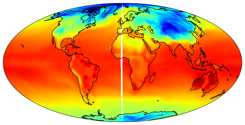
Since the data is periodic in longitude, we need to append a copy to the array. We need to do this since cartopy interpolates data. If we don’t, then there will be missing longitude band of missing data in for plot as shown below:

Lon, Lat = np.meshgrid(ds['lon'].data, ds['lat'].data)

plt.figure(figsize=(15, 5))
ax = plt.axes(projection=ccrs.Mollweide())
ax.set_global()
ax.coastlines()
ax.contourf(Lon, Lat, np.squeeze(decode(GTS)), 200, transform=ccrs.PlateCarree(), cmap='jet')
plt.show()

Fig 1. Global Near surface temperature on a (longitude)-periodic domain.