MERRA-2 Data via NASA’s OPeNDAP in the Cloud.

MERRA-2 Data via NASA’s OPeNDAP in the Cloud.#

Requirements to run this notebook

Have an Earth Data Login account
Preferred method of authentication.

Objectives

Use best practices from OPeNDAP, pydap, and xarray, to

Discover all OPeNDAP URLs associated with a MERRA-2 collection.
Authenticate via EDL (token based)
Explore MERRA-2 collection and filter variables
Consolidate Metadata at the collection level
Download/stream a subset of interest.

Author: Miguel Jimenez-Urias, ‘25

from pydap.net import create_session
from pydap.client import get_cmr_urls, consolidate_metadata, open_url
import xarray as xr
import datetime as dt
import earthaccess
import matplotlib.pyplot as plt
import numpy as np
import pydap

print("xarray version: ", xr.__version__)
print("pydap version: ", pydap.__version__)

xarray version:  2025.9.0
pydap version:  3.5.8

Explore the MERRA-2 Collection#

merra2_doi = "10.5067/VJAFPLI1CSIV" # available e.g. GES DISC MERRA-2 documentation 
                                    # https://disc.gsfc.nasa.gov/datasets/M2T1NXSLV_5.12.4/summary?keywords=MERRA-2
# One month of data
time_range=[dt.datetime(2023, 1, 1), dt.datetime(2023, 2, 28)]

urls = get_cmr_urls(doi=merra2_doi,time_range=time_range, limit=100) # you can incread the limit of results
len(urls)

Authenticate#

To hide the abstraction, we will use earthaccess to authenticate, and create cache session to consolidate all metadata

auth = earthaccess.login(strategy="interactive", persist=True) # you will be promted to add your EDL credentials

# pass Token Authorization to a new Session.
cache_kwargs={'cache_name':'data/MERRA2'}
my_session = create_session(use_cache=True, session=auth.get_session(), cache_kwargs=cache_kwargs)
# my_session.cache.clear()

Explore Variables in collection and filter down to keep only desirable ones#

We do this by specifying the NASA OPeNDAP server to process requests via the DAP4 protocol.

There are two ways to do this:

Use pydap to inspect the metadata (all variables inside the files, and their description). You can run the following code to list all variable names.

from pydap.client import open_url
ds = open_url(url, protocol='dap4', session=my_session)
ds.tree() # this will display the entire tree directory

ds[Varname].attributes # will display all the information about Varname in the remote file.

Use OPeNDAP’s Data Request Form visible from the browser. You accomplish this by taking an OPeNDAP URL, adding the .dmr extension, and paste that resulting URL into a browser.

Either way, you can inspect variable names, their description, without downloading any large arrays.

Below, we assume you know which variables you need.

variables = ['lon', 'lat', 'time', 'T2M', "U2M", "V2M"] # variables of interest
CE = "?dap4.ce="+ "/"+";/".join(variables) # Need to add this string as a query expression to the OPeNDAP URL
new_urls = [url.replace("https", "dap4") + CE for url in urls] # 

Consolidate Metadata#

Aggregating multiple remote files at the collection level requires persistent internet connection. The pydap backend allows to download and store the metadata required by xarray locally as a sqlite3 database, and this database can be used as session manager (for futher downloads). Creating this databaset can be done once, and reused, version controlled, etc. Reusing this database can cut the time to generate the aggregated dataset view from minutes to seconds.

consolidate_metadata(new_urls, session=my_session, concat_dim='time')

datacube has dimensions ['lat[0:1:360]', 'lon[0:1:575]'] , and concat dim: `['time']`

Explore an Individual Remote#

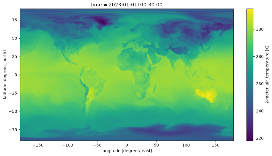
We create an Xarray dataset for visualization purposes. Lets make a plot of near surface Temperature, at a single time unit.

Note

Each granule has 24 time units. Chunking in time as done below when generating the dataset, will ensure the slice is passed to the server. And so subsetting takes place close to the data.

%%time
ds = xr.open_dataset(
    new_urls[0], 
    engine='pydap', 
    session=my_session, 
    chunks={'time':1}, #  <----------- just for now. This instruct the server to subset in time (each granule has 24 times values)
)
ds

CPU times: user 253 ms, sys: 49.4 ms, total: 303 ms
Wall time: 510 ms

<xarray.Dataset> Size: 120MB
Dimensions:  (time: 24, lat: 361, lon: 576)
Coordinates:
  * lon      (lon) float64 5kB -180.0 -179.4 -178.8 -178.1 ... 178.1 178.8 179.4
  * time     (time) datetime64[ns] 192B 2023-01-01T00:30:00 ... 2023-01-01T23...
  * lat      (lat) float64 3kB -90.0 -89.5 -89.0 -88.5 ... 88.5 89.0 89.5 90.0
Data variables:
    T2M      (time, lat, lon) float64 40MB dask.array<chunksize=(1, 361, 576), meta=np.ndarray>
    U2M      (time, lat, lon) float64 40MB dask.array<chunksize=(1, 361, 576), meta=np.ndarray>
    V2M      (time, lat, lon) float64 40MB dask.array<chunksize=(1, 361, 576), meta=np.ndarray>
Attributes: (12/31)
    History:                           Original file generated: Wed Jan 11 21...
    Comment:                           GMAO filename: d5124_m2_jan10.tavg1_2d...
    Filename:                          MERRA2_400.tavg1_2d_slv_Nx.20230101.nc4
    Conventions:                       CF-1
    Institution:                       NASA Global Modeling and Assimilation ...
    References:                        http://gmao.gsfc.nasa.gov
    ...                                ...
    identifier_product_doi:            10.5067/VJAFPLI1CSIV
    RangeBeginningDate:                2023-01-01
    RangeBeginningTime:                00:00:00.000000
    RangeEndingDate:                   2023-01-01
    RangeEndingTime:                   23:59:59.000000
    created:                           2025-01-07T19:36:33Z

Visualize#

In Xarray, when visualizing data, data gets downloaded. By chunking in time when creating the dataset, we ensure in the moment of visualizing a single time-unit in xarray, the time slice is passed to the server. This has the effect of reducing the amount of data downloaded, and faster transfer.

fig, ax = plt.subplots(figsize=(12, 6))
ds['T2M'].isel(time=0).plot();

../_images/f30839d01274c048e0e74fafe5787908e8bf074d9594c4773bdfcceafe251f9b.png

Subset the Aggregated Dataset, while resampling in time#

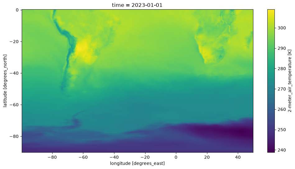
We select data relevant to the Southern Hemisphere, in the area near South America.
Store data in daily averages (as opposed to hourly data).

Note

To accomplish this, we need to identify the slice in index space, and chunk the dataset before streaming. Doing so will ensure spatial subsetting is done on the server side (OPeNDAP) close to the data, while Xarray performs the daily average.

lat, lon = ds['lat'].data, ds['lon'].data

minLon, maxLon = -100, 50 # spatial subset around South America

iLon = np.where((lon>minLon)&(lon < maxLon))[0]
iLat= np.where(lat < 0)[0]

Create Dataset Aggregation, Chunking in Space#

%%time
ds = xr.open_mfdataset(
    new_urls,
    engine='pydap', 
    session=my_session,
    concat_dim='time',
    combine='nested',
    parallel=True,
    chunks={'lon':len(iLon), 'lat': len(iLat)}, #  <----------- This instructs the OPeNDAP server to subset in space
)

CPU times: user 1.21 s, sys: 314 ms, total: 1.52 s
Wall time: 4.5 s

## now subset the Xarray Dataset and rechunk so it is a single chunk
ds = ds.isel(lon=slice(iLon[0], iLon[-1]+1), lat=slice(iLat[0], iLat[-1]+1)).chunk({'lon':len(iLon), 'lat': len(iLat)})
ds

<xarray.Dataset> Size: 1GB
Dimensions:  (time: 1416, lat: 181, lon: 239)
Coordinates:
  * lon      (lon) float64 2kB -99.38 -98.75 -98.12 -97.5 ... 48.12 48.75 49.38
  * time     (time) datetime64[ns] 11kB 2023-01-01T00:30:00 ... 2023-02-28T23...
  * lat      (lat) float64 1kB -90.0 -89.5 -89.0 -88.5 ... -1.0 -0.5 -1.798e-13
Data variables:
    T2M      (time, lat, lon) float64 490MB dask.array<chunksize=(24, 181, 239), meta=np.ndarray>
    U2M      (time, lat, lon) float64 490MB dask.array<chunksize=(24, 181, 239), meta=np.ndarray>
    V2M      (time, lat, lon) float64 490MB dask.array<chunksize=(24, 181, 239), meta=np.ndarray>
Attributes: (12/31)
    History:                           Original file generated: Wed Jan 11 21...
    Comment:                           GMAO filename: d5124_m2_jan10.tavg1_2d...
    Filename:                          MERRA2_400.tavg1_2d_slv_Nx.20230101.nc4
    Conventions:                       CF-1
    Institution:                       NASA Global Modeling and Assimilation ...
    References:                        http://gmao.gsfc.nasa.gov
    ...                                ...
    identifier_product_doi:            10.5067/VJAFPLI1CSIV
    RangeBeginningDate:                2023-01-01
    RangeBeginningTime:                00:00:00.000000
    RangeEndingDate:                   2023-01-01
    RangeEndingTime:                   23:59:59.000000
    created:                           2025-01-07T19:36:33Z

Now, we take the daily average. With xarray, this is done lazily (no actual computation takes place until plotting, or saving data locally)

nds = ds.resample(time="1D").mean()
nds

<xarray.Dataset> Size: 61MB
Dimensions:  (time: 59, lat: 181, lon: 239)
Coordinates:
  * lon      (lon) float64 2kB -99.38 -98.75 -98.12 -97.5 ... 48.12 48.75 49.38
  * lat      (lat) float64 1kB -90.0 -89.5 -89.0 -88.5 ... -1.0 -0.5 -1.798e-13
  * time     (time) datetime64[ns] 472B 2023-01-01 2023-01-02 ... 2023-02-28
Data variables:
    T2M      (time, lat, lon) float64 20MB dask.array<chunksize=(1, 181, 239), meta=np.ndarray>
    U2M      (time, lat, lon) float64 20MB dask.array<chunksize=(1, 181, 239), meta=np.ndarray>
    V2M      (time, lat, lon) float64 20MB dask.array<chunksize=(1, 181, 239), meta=np.ndarray>
Attributes: (12/31)
    History:                           Original file generated: Wed Jan 11 21...
    Comment:                           GMAO filename: d5124_m2_jan10.tavg1_2d...
    Filename:                          MERRA2_400.tavg1_2d_slv_Nx.20230101.nc4
    Conventions:                       CF-1
    Institution:                       NASA Global Modeling and Assimilation ...
    References:                        http://gmao.gsfc.nasa.gov
    ...                                ...
    identifier_product_doi:            10.5067/VJAFPLI1CSIV
    RangeBeginningDate:                2023-01-01
    RangeBeginningTime:                00:00:00.000000
    RangeEndingDate:                   2023-01-01
    RangeEndingTime:                   23:59:59.000000
    created:                           2025-01-07T19:36:33Z

Finally#

Store data locally, as NetCDF4. At this stage:

Data is downloaded (spatially subsetted via OPeNDAP)
Data is resampled (via Xarray)

%%time
nds.to_netcdf("data/Merra2_subset.nc4", mode='w')

CPU times: user 14.1 s, sys: 15.9 s, total: 30 s
Wall time: 3min 28s