Acceso a datos de calidad del aire casi en tiempo real (NRT) de TEMPO mediante OPeNDAP de NASA Earthdata en la nube

Acceso a datos de calidad del aire casi en tiempo real (NRT) de TEMPO mediante OPeNDAP de NASA Earthdata en la nube#

Los archivos de dióxido de nitrógeno Nivel 2 (PROVISIONAL) proporcionan información de gases traza a la resolución espacial nativa de TEMPO, ~10 km^2 en el centro del Field of Regard (FOR), para gránulos individuales. Cada gránulo cubre todo el FOR Norte-Sur de TEMPO, pero solo una parte del FOR Este-Oeste. Fuente: NASA Earthdata.

Requisitos#

Autenticación EDL (usuario/contraseña)
python>=3.12.

Objetivos#

Descarga un archivo remoto con (sub)selection#

a) Por variables
b) Por coordenadas geograficas

Descarga de múltiples archivos remotos#

A cada archivo se le aplica la subseleccion de una subregion de datos de interes antes de descargar.

Referencias#

Liu, X. (2025). TEMPO NO2 tropospheric, stratospheric, and total columns V04 [Data set]. NASA Langley Atmospheric Science Data Center Distributed Active Archive Center. https://doi.org/10.5067/IS-40E/TEMPO/NO2_L2.004

import xarray as xr
import datetime as dt
import earthaccess
import pydap
import matplotlib.pyplot as plt
import numpy as np

# import pydap-specific tools
from pydap.net import create_session
from pydap.client import get_cmr_urls, open_url
from pydap.client import to_netcdf as dap_to_netcdf

Como encontrar URLs de OPeNDAP#

Usando la API CMR de NASA#

Consultamos el Common Metadata Repository (CMR por sus siglas en ingles) de la NASA para identificar archivos remotos. Nos interesan datos de TEMPO NO2 tropospheric and stratospheric columns V04. Esta colección proporciona datos horarios para datos de nivel 2, considerados Near Real Time (NRT).

TEMPO_L2_NRTNO2_ccid = "C3685896872-LARC_CLOUD" # 
time_range = [dt.datetime(2025, 10, 1), dt.datetime(2025, 10, 7)] # One month of data

bounding_box = [-124.63309,46.35932,  -121, 49.83307] # WSEN area within Seattle PNW

cmr_urls = get_cmr_urls(ccid=TEMPO_L2_NRTNO2_ccid, bounding_box=bounding_box, time_range=time_range, limit=1000) # you can incread the limit of results

print("################################################ \n We found a total of ", len(cmr_urls), "OPeNDAP URLS!!!\n################################################")

################################################ 
 We found a total of  73 OPeNDAP URLS!!!
################################################

cmr_urls[:5]

['https://opendap.earthdata.nasa.gov/collections/C3685896872-LARC_CLOUD/granules/TEMPO_NO2_L2_V04_20251001T141426Z_S004G08.nc',
 'https://opendap.earthdata.nasa.gov/collections/C3685896872-LARC_CLOUD/granules/TEMPO_NO2_L2_V04_20251001T151426Z_S005G08.nc',
 'https://opendap.earthdata.nasa.gov/collections/C3685896872-LARC_CLOUD/granules/TEMPO_NO2_L2_V04_20251001T161426Z_S006G08.nc',
 'https://opendap.earthdata.nasa.gov/collections/C3685896872-LARC_CLOUD/granules/TEMPO_NO2_L2_V04_20251001T171426Z_S007G08.nc',
 'https://opendap.earthdata.nasa.gov/collections/C3685896872-LARC_CLOUD/granules/TEMPO_NO2_L2_V04_20251001T181426Z_S008G08.nc']

Autenticación EDL mediante earthaccess y OPeNDAP#

Puedes autenticarte mediante earthaccess como se muestra a continuacion. Debes tener una cuenta EDL válida. Hay dos estrategias para autenticarte con earthaccess:

strategy="interactive". Esto pedirá tu usuario y contraseña de EDL.
strategy="netrc". Usa esta opción si el notebook se ejecuta en un entorno donde se puede recuperar un .netrc con tus credenciales.

A continuación, el valor predeterminado será netrc, asumiendo que el usuario ejecutó el notebook Authenticate.ipynb. Si no es así, puedes cambiar la estrategia a "interactive".

from earthaccess.exceptions import LoginStrategyUnavailable
try:
    auth = earthaccess.login(strategy="netrc", persist=True) # you will be promted to add your EDL credentials
except LoginStrategyUnavailable:
    auth = earthaccess.login(strategy="interactive", persist=True)

# pass Token Authorization to a new Session.
my_session = create_session(auth.get_session())

Acceso solo a metadatos con PyDAP#

Podemos acceder a metadatos producidos por OPeNDAP para identificar las variables de interés. En particular, aquellas asociadas con valores de latitud y longitud.

A continuación necesitamos solicitar los metadatos DAP4 al servidor remoto.

%%time
pyds = open_url(cmr_urls[0],protocol="dap4", session=my_session)
pyds.tree()

.TEMPO_NO2_L2_V04_20251001T141426Z_S004G08.nc
├──product
│  ├──main_data_quality_flag
│  ├──vertical_column_troposphere
│  ├──vertical_column_stratosphere
│  └──vertical_column_troposphere_uncertainty
├──geolocation
│  ├──time
│  ├──longitude
│  ├──latitude
│  ├──solar_azimuth_angle
│  ├──longitude_bounds
│  ├──solar_zenith_angle
│  ├──viewing_zenith_angle
│  ├──latitude_bounds
│  ├──relative_azimuth_angle
│  └──viewing_azimuth_angle
├──support_data
│  ├──surface_pressure
│  ├──wind_speed
│  ├──amf_cloud_pressure
│  ├──vertical_column_total_uncertainty
│  ├──vertical_column_total
│  ├──terrain_height
│  ├──fitted_slant_column_uncertainty
│  ├──amf_troposphere
│  ├──fitted_slant_column
│  ├──gas_profile
│  ├──fitted_slant_column_uncorrected
│  ├──amf_cloud_fraction
│  ├──snow_ice_fraction
│  ├──amf_diagnostic_flag
│  ├──destriping_correction
│  ├──albedo
│  ├──amf_total
│  ├──scattering_weights
│  ├──tropopause_pressure
│  ├──eff_cloud_fraction
│  ├──amf_stratosphere_clear_sky
│  ├──pbl_height
│  ├──amf_total_clear_sky
│  ├──temperature_profile
│  ├──amf_stratosphere
│  ├──amf_troposphere_clear_sky
│  ├──scattering_weights_clear_sky
│  └──ground_pixel_quality_flag
├──qa_statistics
│  ├──fit_rms_residual
│  └──fit_convergence_flag
├──xtrack
└──mirror_step
CPU times: user 151 ms, sys: 20.6 ms, total: 172 ms
Wall time: 2.55 s

dims = list(set(pyds['geolocation/latitude'].dims + pyds['geolocation/longitude'].dims + pyds['geolocation/time'].dims))

print("\nnecessary dimensions to download:", dims, "\n")

necessary dimensions to download: ['/xtrack', '/mirror_step']

Subdividir por nombres de variables#

Primero exploramos solo las coordenadas y sus dimensiones, para identificar el subconjunto espacial.

output_path = "data/"

Transmitir datos#

Cada archivo remoto se almacena en un archivo individual. No hay agregación de datos.

%%time
dap_to_netcdf(cmr_urls, session=my_session, 
              keep_variables= dims + [
                                      "/geolocation/time",
                                      "/geolocation/longitude",
                                      "/geolocation/latitude", 
              ],
              output_path=output_path)

CPU times: user 163 ms, sys: 249 ms, total: 412 ms
Wall time: 10.4 s

Inspeccionar todos los archivos descargados#

Aquí identificamos con más detalle el subconjunto de datos necesario en el archivo remoto, que devolverá SOLO datos dentro de nuestra caja delimitadora, para cualquier variable de interés posible.

%%time
# Use coord data from Bounding Box
minLon, maxLon = bounding_box[0], bounding_box[2]
minLat, maxLat = bounding_box[1], bounding_box[3]

slices = []
# iterate over all downloaded files
# Will use the URL to extract the filename
for url in cmr_urls:
    filename = output_path+f"{url.split('/')[-1][:-3]}.nc4"
    # Flatten data 
    ds = xr.merge([xr.open_dataset(filename), xr.open_dataset(filename, group='geolocation')])
    ds.load()
    # Identify subset from Lon/Lat data per granule
    
    longitude = ds['longitude'].values
    latitude = ds['latitude'].values

    mask = (
        (longitude >= minLon) & (longitude <= maxLon) &
        (latitude >= minLat) & (latitude <= maxLat)
    )

    rows, cols = np.where(mask)
    # indexes below
    y0, y1 = rows.min(), rows.max()
    x0, x1 = cols.min(), cols.max()
    slice_ = {
        "mirror_step":(y0,y1),
        "xtrack": (x0,x1),
        }
    slices.append({
        "mirror_step":(y0,y1),
        "xtrack": (x0,x1),
        })

CPU times: user 477 ms, sys: 127 ms, total: 604 ms
Wall time: 613 ms

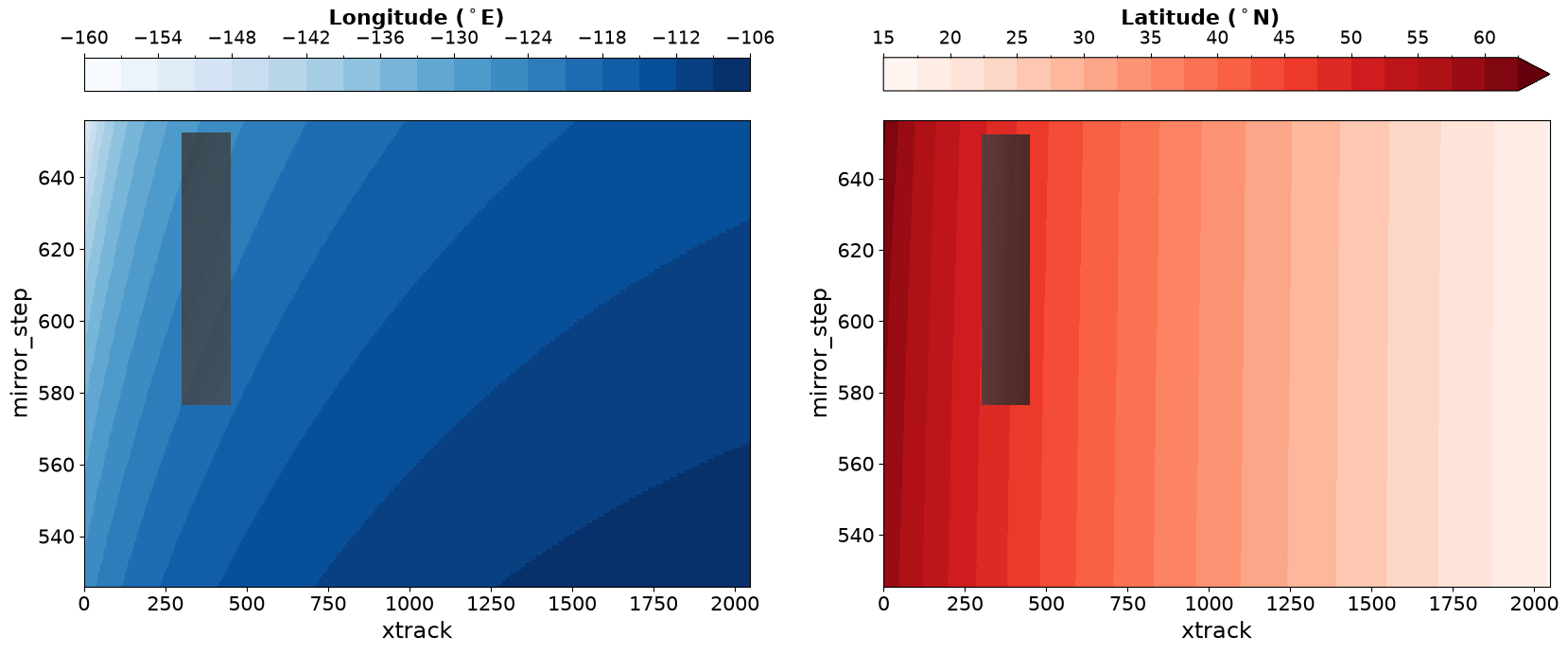
Visualizar coordenadas#

Será necesario enmascarar arreglos para visualizar,

Graficar solo el último gránulo.

Lon = ds['longitude'].isel(mirror_step=slice(y0, y1), xtrack=slice(x0, x1))

Lon_masked = xr.full_like(ds['longitude'], np.nan)
Lon_masked.loc[dict(
    mirror_step=Lon['mirror_step'],
    xtrack=Lon['xtrack']
)] = Lon


Lat = ds['latitude'].isel(mirror_step=slice(y0, y1), xtrack=slice(x0, x1))
Lat_masked = xr.full_like(ds['latitude'], np.nan)
Lat_masked.loc[dict(
    mirror_step=Lat['mirror_step'],
    xtrack=Lat['xtrack']
)] = Lat

fig, axes = plt.subplots(figsize=(20,8), ncols=2)
pbar_lon = ds['longitude'].plot(ax=axes[0], cmap="Blues", vmin=-160, vmax=-105, levels=np.arange(-160,-105,3), cbar_kwargs={"location": "top"})
pbar_lon.colorbar.ax.tick_params(labelsize=14)
pbar_lon.colorbar.set_label(r'Longitude ($^\circ$E)', fontsize=16, weight='bold')
Lon_masked.plot(ax=axes[0], cmap="Greys_r",vmin=-160,vmax=20, add_colorbar=False, alpha=0.8)

# Optional: Set limits if not automatically handling it
axes[0].set_xlim([ds['xtrack'].min(),ds['xtrack'].max()])
axes[0].set_ylim([ds['mirror_step'].min(),ds['mirror_step'].max()])

pbar_lat = ds['latitude'].plot(ax=axes[1], vmin=15, vmax=62.5, levels=20, cmap='Reds',cbar_kwargs={"location": "top"})
pbar_lat.colorbar.ax.tick_params(labelsize=14)
pbar_lat.colorbar.set_label(r'Latitude ($^\circ$N)', fontsize=16, weight='bold')
Lat_masked.plot(ax=axes[1], cmap="Greys_r",vmin=40,vmax=90, add_colorbar=False, alpha=0.8)


plt.setp(axes[0].get_xticklabels(), fontsize=15)
plt.setp(axes[0].get_yticklabels(), fontsize=15)
axes[0].set_xlabel('xtrack', fontsize=17.5)
axes[0].set_ylabel('mirror_step', fontsize=17.5)

plt.setp(axes[1].get_xticklabels(), fontsize=15)
plt.setp(axes[1].get_yticklabels(), fontsize=15);
axes[1].set_xlabel('xtrack', fontsize=17.5)
axes[1].set_ylabel('mirror_step', fontsize=17.5)
plt.show()

../_images/e925d8a298798ca5a55cc9d3630dc376ddff750466de94b8acbc2ba5dc3428ee.png

Ahora definir todas las variables para descargar#

Vars = dims + [
    "/product/main_data_quality_flag",
    "/product/vertical_column_troposphere",
    "/product/vertical_column_stratosphere",
    "/geolocation/time",
    "/geolocation/longitude",
    "/geolocation/latitude",
    "/support_data/wind_speed",
    "/support_data/terrain_height",
    "/support_data/gas_profile",
    "/support_data/pbl_height",
    "/support_data/temperature_profile",
]